Why transition metal discovery still feels slow
You can run a huge number of simulations or robotized experiments, yet transition-metal discovery still often feels like moving one careful step at a time. A catalyst “hit” on paper can fail once the solvent changes, a trace impurity appears, or the metal switches spin state and follows a different pathway than expected.
The search space is also unusually wide: many oxidation states, coordination geometries, ligands, and competing reactions can produce similar-looking outcomes. Small structural tweaks can flip selectivity or stability, so teams end up iterating cautiously instead of scaling blindly.
Even before AI enters the picture, the bottlenecks are practical: synthesizing air-sensitive complexes, running controlled kinetics, and getting reproducible characterization. Those steps cost time, specialized staff, and instrument hours, and they don’t compress just because screening is faster.
What “AI speeding discovery” actually means in the lab
A familiar pattern in metal programs is that the “slow” part isn’t generating ideas, it’s deciding which 20 ideas deserve the next two weeks of synthesis and characterization. In practice, AI usually speeds discovery by moving that decision upstream: ranking candidate ligands, oxidation states, supports, or reaction conditions so the lab runs fewer low-information experiments and fewer expensive DFT calculations.
That looks like triage and prioritization rather than automation. A model might predict relative trends (stability, spin state likelihood, binding energies, selectivity proxies) and flag regions of chemical space that are probably dead ends. The payoff is measured in hit rate and cycle time: how many iterations to reach a viable complex, how often predictions reproduce across batches, and whether “top picks” still perform when solvent, impurities, or scale changes. The models rarely remove the need for careful synthesis and standardized assays; they mostly reduce wasted runs.
The hidden constraint: getting usable data for metals
A common frustration is that transition-metal work produces a lot of “results” but not a lot of reusable data. Papers and lab notebooks often report yields, selectivities, or a single turnover number under one set of conditions, while the model needs inputs that are comparable across ligands, oxidation states, and assay setups. Metals also bring measurement ambiguity: mixtures of species, solvent and counterion effects, batch-to-batch impurities, and speciation that changes during the run.
Even when you have DFT data, you may not have the right kind. Different functionals, spin treatments, solvation models, and convergence settings can shift energies enough to scramble rankings, which is exactly what screening depends on. Building a dataset that a model can learn from usually means paying for consistency: standardized protocols, metadata (water content, atmosphere, temperature profiles), and negative results. That effort is unglamorous and expensive, but it often determines whether “AI acceleration” shows up outside a slide deck.
How you represent a metal complex changes everything
Two teams can study the “same” complex and still feed very different inputs into a model. One representation treats it like a flat graph of atoms and bonds; another encodes 3D geometry, partial charges, and the metal’s local environment; a third skips structure and uses hand-built descriptors like ligand field strength or donor counts. For organic molecules, these choices often converge. For transition metals, they can diverge sharply because the metal–ligand picture depends on spin state, oxidation state, coordination changes, and multiple plausible isomers.
The practical consequence is that a model may look accurate while quietly learning shortcuts: “chlorides usually underperform,” or “square-planar often means X,” without actually tracking the active species. Richer representations can help, but they cost more—conformer generation, DFT geometries, and careful annotation—and they can still be wrong if the catalyst rearranges under reaction conditions.
Choosing models: fast screening vs faithful physics
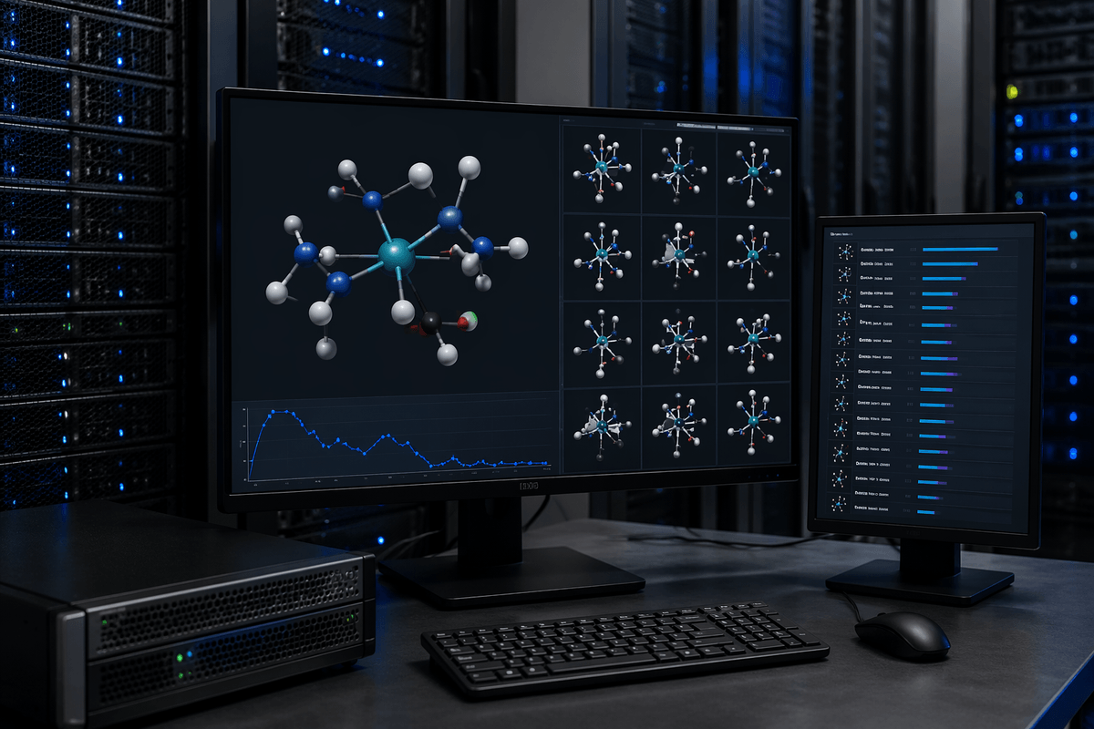
A practical choice shows up as soon as you start ranking candidates: do you want a model that is cheap enough to score 100,000 complexes, or one that respects the chemistry closely enough to be trusted on the top 50? Fast screeners—simple descriptor models, many graph networks, or models trained on coarse DFT targets—can be great at ordering “more like known winners” vs “probably irrelevant,” especially within a narrow ligand family. They also fail quietly when the program changes metal, oxidation state, or mechanism, because the training signal rarely covers that shift.
More faithful approaches push toward physics-aware features (3D, local environments), higher-quality reference data, or hybrid workflows where ML proposes candidates and DFT re-ranks the shortlist. That usually improves transfer and interpretability, but the cost moves back into the loop: geometry generation, spin-state enumeration, and compute time. Many teams end up with a two-stage pipeline: a fast filter to avoid wasting synthesis, then a slower check to avoid chasing a brittle trend.
Closing the loop with experiments: active learning workflows
Most groups eventually discover that a ranking model is only as useful as its ability to learn from what the bench actually saw last week. Active learning turns that into a workflow: start with a small, well-characterized set of complexes, train a model, then choose the next experiments based on where the model is uncertain, where a prediction would change the decision, or where two candidate mechanisms are hard to distinguish. The goal is not “more data,” but more informative data per synthesis and assay hour.
In metal programs, the loop often includes cheap proxies (stability in air, ligand substitution rates, solubility, basic activity screens) before committing to full kinetics, operando characterization, or higher-level DFT. A practical difficulty is that the loop breaks when experiments can’t be run in a standardized way: subtle differences in water content, catalyst activation, or mixing can dominate the signal and teach the model the lab’s noise. The best implementations treat protocols and metadata as first-class outputs, because the model needs repeatable feedback to improve.
Trust and failure modes: uncertainty, bias, and surprises
A common moment of doubt is when the model “confidently” ranks a complex that a chemist would never bother making. That usually isn’t AI being reckless; it’s a mismatch between the question you asked (“score candidates like the training set”) and the question you meant (“work under my exact activation and assay conditions”). Calibration matters: you want uncertainty that tracks reality, so a high score with high uncertainty is treated like a hypothesis, not a decision.
Bias shows up in unromantic places. If the dataset overrepresents stable, easy-to-make chloride salts, the model may quietly prefer them even when the program needs fragile, unusual precatalysts. Negative results are another trap: if “failed synthesis” or “decomposed in glovebox transfer” never makes it into the data, the model learns a world without those costs.
Surprises are guaranteed because the active species may not be the drawn complex. Spin-state flips, ligand exchange, nanoparticle formation, or trace poisons can dominate outcomes, and the model can’t predict what wasn’t measured. The practical safeguard is to design early experiments that distinguish mechanisms and to treat out-of-distribution flags as reasons to slow down, not push harder.
What to do next if you want to apply this
A familiar starting point is a single decision you already make repeatedly: which candidates are worth synthesis time. Define one measurable target (or a small set) and the “costs” that matter alongside performance—air stability, availability of ligands, glovebox time, assay throughput—because an AI ranker that ignores those will optimize the wrong thing.
Audit what you truly have: not papers, but a table with structures, conditions, metadata, and explicit failures. If that table is thin or inconsistent, invest first in standardizing protocols and capturing negatives; it’s slower than buying a model, but it’s usually the gating step.
Run a two-stage pilot. Use a cheap model to filter broadly, then re-rank a shortlist with higher-fidelity DFT and a small, tightly controlled experiment loop. Judge success by cycle time, hit rate, and reproducibility across batches—not by a single accuracy metric on yesterday’s dataset.